Data Mining and Knowledge Discovery, 2017, vol. 31(6), pp.1793-1839
poster
pre-print
Visual Analysis of Pressure in Football
Gennady Andrienko1,2, Natalia Andrienko1,2, Guido Budziak3,
Jason Dykes2, Georg Fuchs1, Tatiana von Landesberger4
and Hendrik Weber5
1 Fraunhofer Institute for Intelligent Analysis and Information Systems IAIS
Schloss Birlighoven, 53757 Sankt Augustin, Germany
2 City University London
Northampton Square, London EC1V OHB, United Kingdom
3 TU Eindhoven, The Netherlands
4 TU Darmstadt, Germany
5 DFL Deutsche Fussball Liga GmbH, Germany
Abstract.
Modern movement tracking technologies enable acquisition of high
quality data about movements of the players and the ball in the course of
a football match. However, there is a large distance between the raw data
and the insights into team behaviors that analysts would like to gain. To
enable such insights, it is necessary first to establish relationships between the
concepts characterizing behaviors and what can be extracted from data. This
task is challenging since the concepts are not strictly defined. We propose
a computational approach to detecting and quantifying the relationships of
pressure emerging during a game. Pressure is exerted by defending players
upon the ball and the opponents. Pressing behavior of a team consists of
multiple instances of pressure exerted by the team members. The extracted
pressure relationships can be analyzed in detailed and summarized forms. We
support the analysis by static and dynamic visualizations and by interactive
query tools. We describe the methods and tools for pressure analysis we have
developed and give examples of applying these methods and tools to real data
from games of German Bundesliga, where the teams actively used pressing in
their defense tactics.
On this page you can access high-resolution versions of the figures contained in the paper.

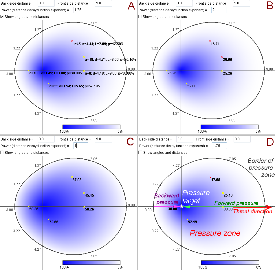
Figure 1. The shape of a pressure zone and the distribution of the pressure levels. The variation of the pressure levels within the pressure zone is represented by varying the color saturation from fully saturated blue for 100% pressure to fully unsaturated (i.e., white) for zero pressure. The pressure levels in five selected points are shown by numbers. The images demonstrate the effect of using different exponents for the distance decay function: 1.75 (A and D), 2 (B), and 1 (C).}
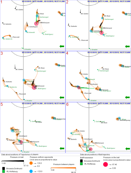
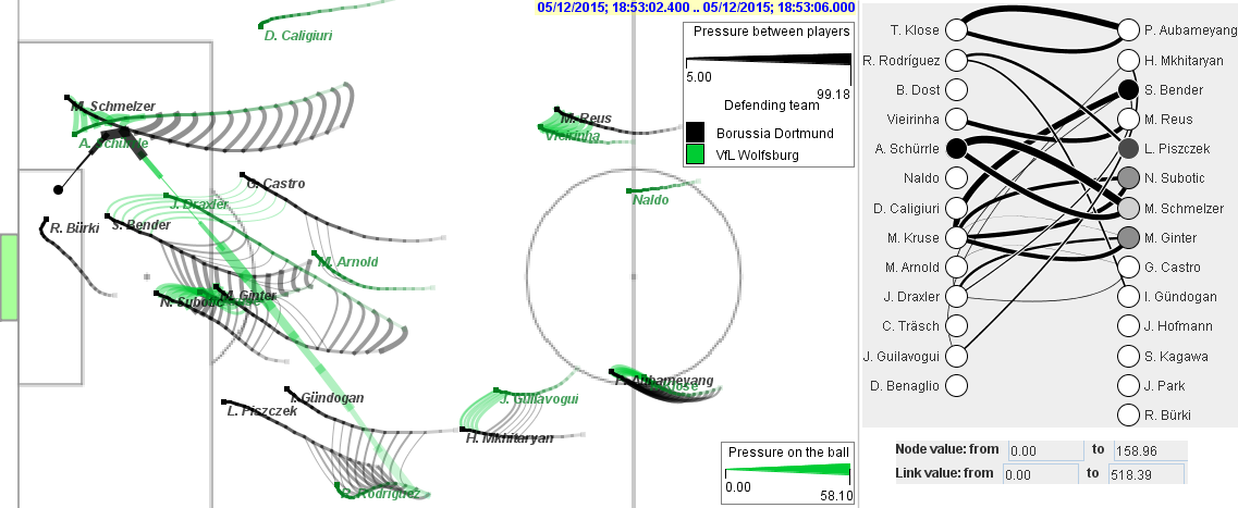
Figure 2. Development of a game episode involving pressure on the ball and on players of
the attacking team, namely, VfL Wolfsburg. The green arrows in the lower right corners of
the images indicate the attack direction of VfL Wolfsburg. The circles in orange and blue
represent positive and negative values of pressure between players, i.e., pressure exerted by
players of the defending team (Borussia Dortmund) and pressure received by players of the
attacking team. The sizes of the red circles represent the cumulative pressure on the ball.
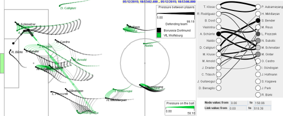
Figure 3. Left: Player-to-player pressure is visually represented on a map by curved linear symbols. Right: For this game episode, a pressure graph shows the total amounts of pressure from the players on the ball (by node darkness) and on the opponents (by line widths).
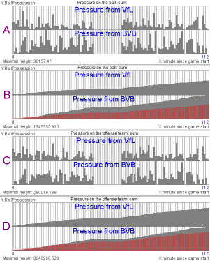
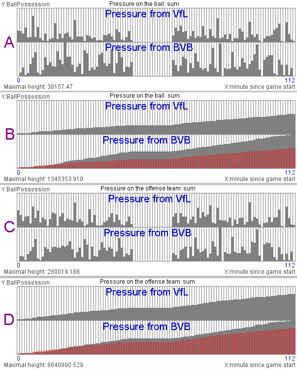
Figure 4. Two-dimensional (2D) time histograms show he amounts of the pressure on the
ball (A, B) and opponents (C, D) summarized by 1-minute time intervals. The horizontal
dimension represents time. Each 2D histogram shows the pressure exerted by two teams,
VfL in the upper row and BvB in the lower row. In histograms B and D, the amounts of
pressure are accumulated along the time axis.
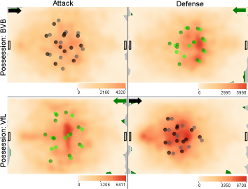
Figure 5. Density maps represent the spatial distributions of the field players (goalkeepers
excluded) of BVB and VfL during the ball possession by BVB (top) and VfL (bottom).
Darker shading means higher density. The dot symbols show the average positions of the
field players in the first (lighter dots) and second (darker dots) halves of the game. The
arrows show the attack directions of the teams.
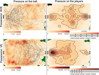
Figure 6. Spatial summaries of the pressure on the ball (left) and on the players (right) during
the ball possession by BVB (top) and VfL (bottom). On the left, the amount of pressure
on the ball is shown by shading; darker shades mean more pressure. The gray lines overlaid
upon the shading show the ball movements when there was no pressure. On the right,
the amount of pressure on the players is shown by shading and, additionally, by isolines
connecting points with the same pressure values.
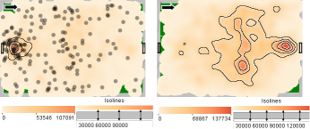
Figure 7. Left: the pressure of VfL on BVB players in the first 3 seconds after BVB gained the
ball. The dots show the locations of the events of ball re-gain by BVB. Right: the pressure
of VfL on BVB players in the remaining time.
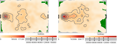
Figure 8. The pressure of BVB on VFL players in the first and second halves of the game.
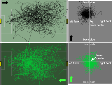
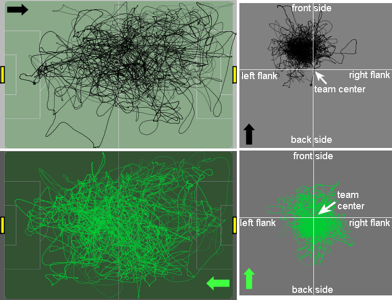
Figure 9. Transformation of players' absolute positions to relative positions within their teams
is illustrated by example of selected trajectories of two players, one from BVB (top) and
another from VfL (bottom).
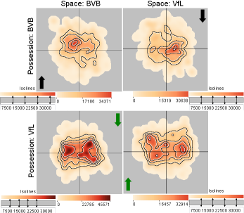
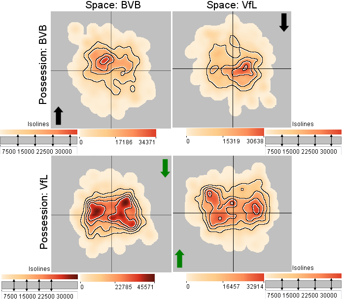
Figure 10. Distribution of the amounts of pressure on the ball in the spaces of the teams BVB
(left) and VfV (right) in situations of ball possession by BVB (top) and VfL (bottom). The
arrows indicate the attack direction in each group of situations. The colors of the arrows
indicate the attacking teams: black for BVB and green for VfL. The pressure on the ball is
generated by the defending teams.
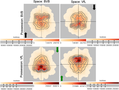
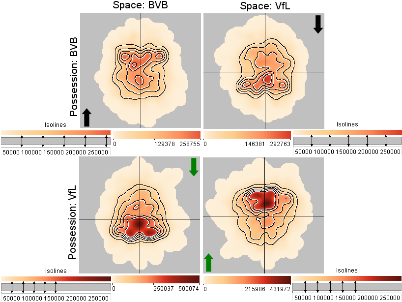
Figure 11. Distribution of the amounts of pressure on the players of the ball possessing teams
in the spaces of the teams BVB (left) and VfL (right) in situations of ball possession by BVB
(top) and VfL (bottom). The arrows have the same meaning as in Fig. 10. The pressure on
the attacking teams is generated by the defending teams.
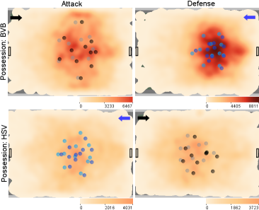
Figure 12. Density of players' positions and team formations of BVB and HSV during the ball
possession by BVB (top) and HSV (bottom). The lighter and darker dots show the average
players' positions in the first and second halves of the game, respectively.
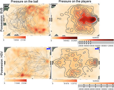
Figure 13. Spatial summaries of the pressure on the ball (left) and on the players (right)
during the ball possession by BVB (top) and HSV (bottom).
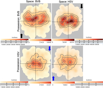
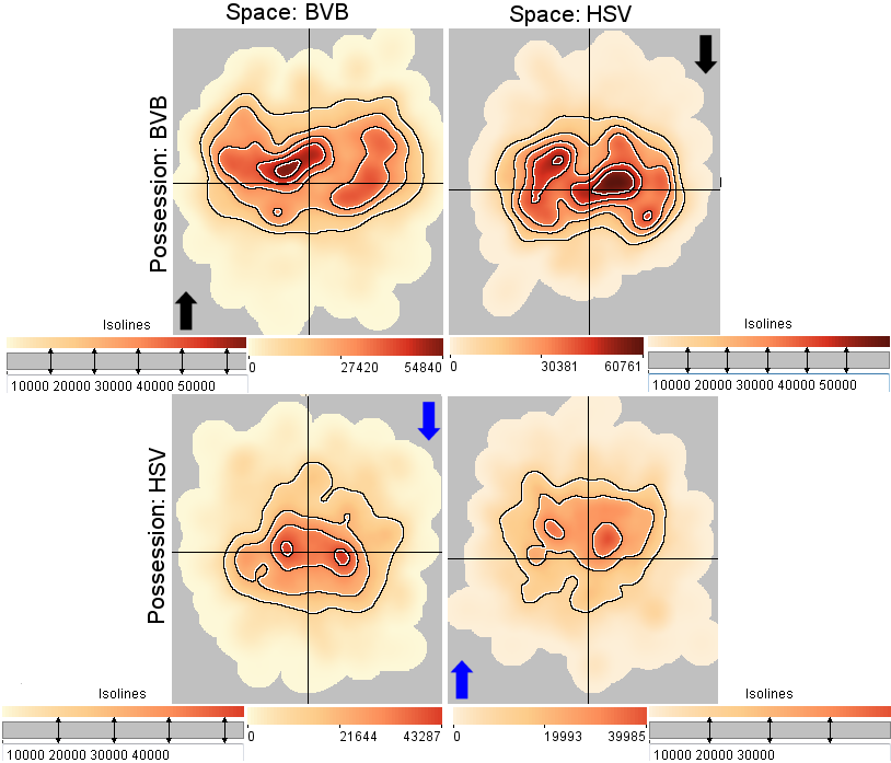
Figure 14. Distribution of the amounts of pressure on the ball in the spaces of the teams BVB
(left) and HSV (right) in situations of ball possession by BVB (top) and HSV (bottom). The
arrows indicate the attack direction in each group of situations. The colors of the arrows
indicate the attacking teams: black for BVB and blue for HSV.
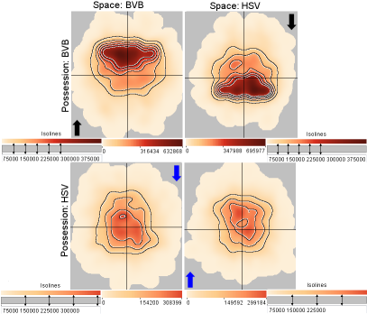
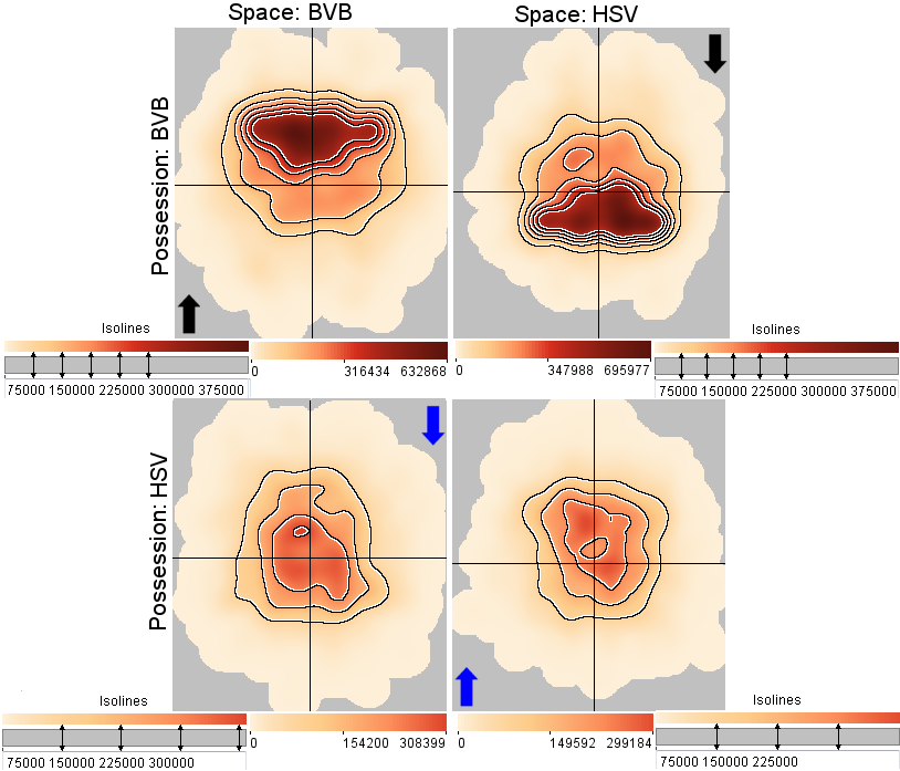
Figure 15. Distribution of the amounts of pressure on the players of the ball possessing teams
in the spaces of the teams BVB (left) and HSV (right) in situations of ball possession by
BVB (top) and HSV (bottom). The arrows have the same meaning as in Fig. 14.

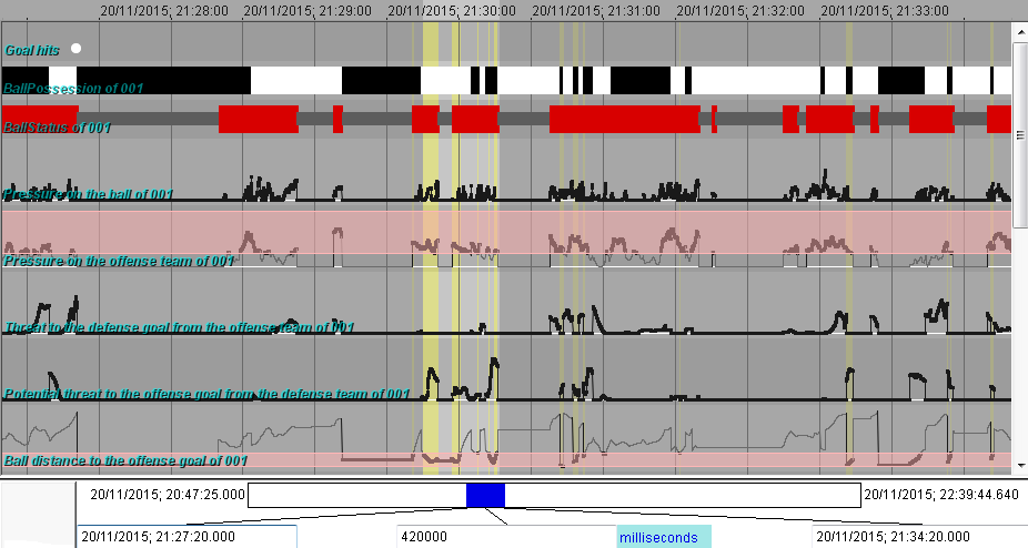
Figure 16. An interactive display of time series of various attributes allows the user to set query conditions and select interesting game episodes for replaying.
A short video demonstrating interactive selection of a game episode based on its characteristics and visual inspection of its dynamics.
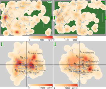
Figure 17. Summaries of the pressure on the ball by BVB in the game against VfL in the last
second before re-gaining the ball in the first (left) and second (right) halves of the game.
The upper images show the distribution of the pressure in the pitch space and the lower
images show the same in the team space of BVB, where the average positions of the BVB
players in the selected time intervals are represented by labeled dots. The blue lines show
the movements of the ball during the selected intervals.
Detailed statistics of pressure in 4 games: 4games_statistics.xlsx
Published online: March 7, 2016;
Last updated: July 25, 2016