Clustering of time intervals is applied to results of spatio-temporal aggregation of eye movement data. Before that, it is reasonable to transform the time references to the common start and end times, i.e., to relative times with respect to the total duration of task fulfillment. The data are aggregated by small time intervals, for example, 1-2% of the total duration of the task completion.
For the clustering, each time interval is represented by a feature vector consisting of values of aggregate attributes referring to the generalized places (areas of interest) or attributes referring to the connections between the places (flows). Any partition-based clustering algorithm can be applied to these feature vectors, for example, the k-means method from the Weka library (www.cs.waikato.ac.nz/ml/weka/). The method uses the Euclidean distance between feature vectors as the measure of dissimilarity.
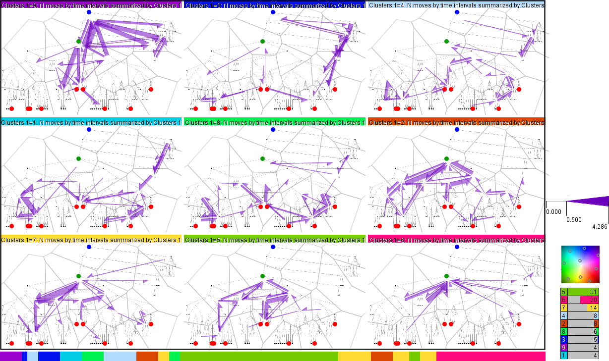
The goal of this analysis is to divide the whole time of task fulfillment into intervals so that the intervals correspond to different kinds of activities, such as tracing the tree perimeter, exploring subtrees, tracing branches by following the links, and checking the candidate solution. For this purpose, the data are aggregated by small time intervals (e.g. 1% length of the task duration). Then the combinations of time-dependent attribute values associated with the connections (flows) between the places are taken as feature vectors describing the time intervals. Thus, for each time interval and each connection there is a corresponding count of eye movements. The vector consisting of the counts for all connections is taken as the feature vector of this time interval. These feature vectors are used to cluster the small time intervals. Several consecutive small intervals having similar feature vectors will be united into longer time intervals. However, non-contiguous time clusters can also be obtained. This may mean that different types of activities are not performed in a strict order or in the same order by all users.
The results of the clustering can be visualized on small multiple flow maps as shown below. The maps summarize the eye movements in the time clusters by representing the average values of the attribute that was used for the clustering; i.e., for each connection and each time cluster, the mean of the values from the time intervals included in the cluster is computed. The attribute means are represented by visual features of the flow symbols, i.e., by widths or color coding.
The image below illustrates the approach. We have aggregated the data by time intervals of 1% of the task duration. Then we applied k-means clustering algorithm to the vectors of the move counts corresponding to the time intervals. We tested different values of the parameter k (number of clusters) for obtaining well discriminable and interpretable spatial patterns. The image shows the results for k=9. Lower values of k mix some of the patterns observable with k=9 and higher values reveal finer differences but not additional types of activities. The colored caption of each map signifies the time cluster represented by the map; the colors have been obtained by projecting the cluster centers onto a two-dimensional color space as illustrated on the right. The temporal positions of the clusters are shown by the segmented bar at the bottom of the figure. The sizes (i.e., total durations) of the time clusters are given in the table in the lower right corner.
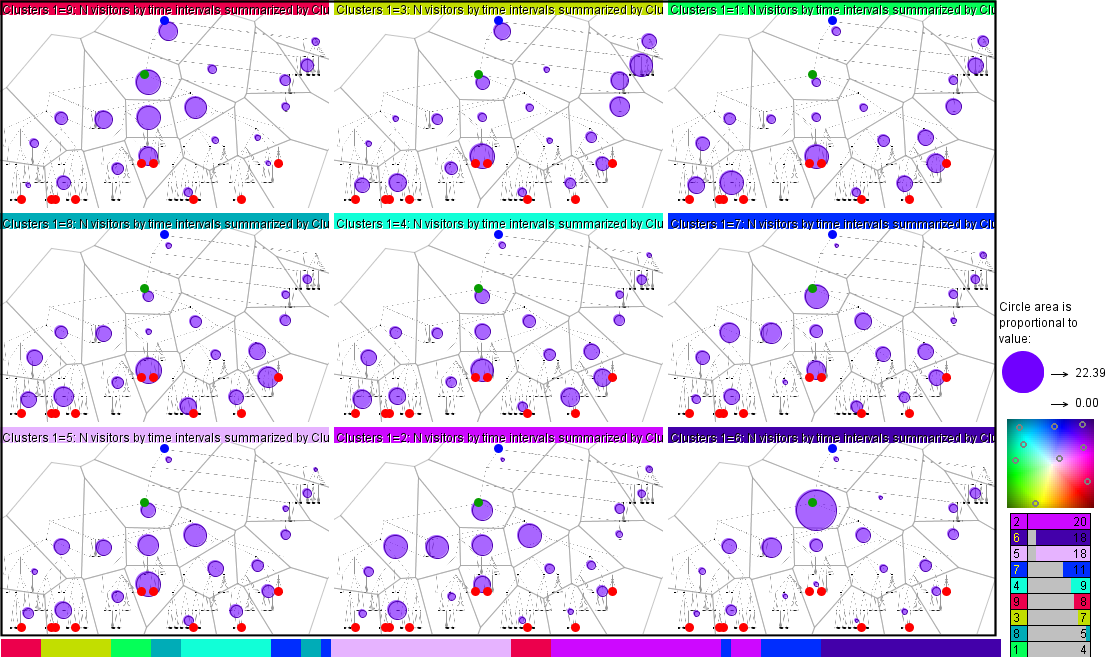
The goal of this analysis is to divide the whole time of task fulfillment into intervals so that the intervals correspond to different patterns of the distribution of the users' attention over the visual stimulus. Technically it is done analogously to the clustering by the similarity of the flows. The difference is that attributes related to the places (areas of interest) are used instead of attributes related to the connections. The data are aggregated by small time intervals (e.g. 1% length of the task fulfillment time). Then the combinations of time-dependent attribute values associated with the places are taken as feature vectors describing the time intervals. For instance, for each time interval and each place there is a corresponding count of place visits. The vector consisting of the counts for all places is taken as the feature vector of this time interval. These feature vectors are used to cluster the small time intervals. Several consecutive small intervals having similar feature vectors will be united into longer time intervals. However, non-contiguous time clusters can also be obtained, indicating re-occurrence of similar attention distribution patterns.
Like in the analysis based on the flows, the time clusters are summarized by computing the means of the attribute values over the time intervals within the clusters; i.e., for each place and each time cluster, the mean of the values from the time intervals included in the cluster is computed. The results are visualized on small multiple attention maps where each map corresponds to one time cluster. The attribute means are represented by coloring or shading of the areas or by proportionally sized symbols or diagrams.
An illustration is given in the image below. The average counts of different users who attended the places are represented by circles with proportional sizes (areas). The counts have been summarized by time clusters obtained by applying the clustering tool to the feature vectors composed of the user counts by the places and time intervals of 1% of the task fulfillment time. The colored caption of each map signifies the time cluster represented by the map; the colors have been obtained by projecting the cluster centers onto a two-dimensional color space as illustrated on the right. The temporal positions of the clusters are shown by the segmented bar at the bottom of the figure. We see that at the beginning most users looked in the middle of the tree diagram and at the root, then their attention switched to the leaves, then they focused more on the marked leaves, then the attention foci gradually moved to the upper tree levels until converging at the target node.