
Flow maps represent results of discrete spatial and spatio-temporal aggregation of trajectories. A flow is an aggregate of multiple movements from one location to another. For eye movement data, a flow may represent the count of eye moves between two areas of interest, or the number of different users that moved their eyes between the two areas, or the average number of eye moves per user, or the maximal number of repeated moves, etc. A flow can be seen as a vector connecting two locations and associated with one or more aggregate attributes derived from the individual movements that have been summarized. Flows can be visually represented in an origin-destination matrix or in a flow map.
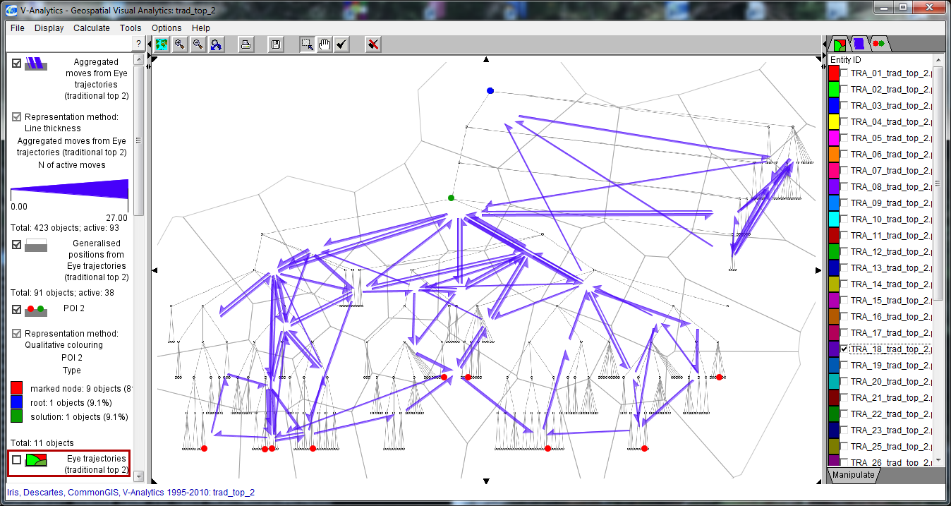
In a flow map, places are connected by special flow symbols varying in widths proportionally to values of an aggregate attribute, such as the total count of moves between the places. Coloring or shading of the symbols can also be employed. In our implementation, flow symbols may have the form of a half of an arrow pointing in the direction of the movement. This shape allows us to represent flows between two places in two opposite directions. There are many intersections among the flow symbols, which clutter the display. This is a consequence of the discontinuous, inertialess character of eye movements: the flows reflect eye jumps from place to place without attending intermediate places. The view can be made clearer by focusing on subsets of flows selected according to the magnitude, length, origin, destination, and/or direction. In the image below, minor flows representing fewer than 3 moves have been filtered out.
Interactive operations: zooming and panning; filtering of flows by attribute values; filtering of trajectories resulting in dynamic re-computing of the aggregate attributes and subsequent map update to reflect the changes (dynamic aggregation).
Dynamic aggregation means dynamic re-computation of the aggregate attributes of the places and flows in response to any filter applied to the trajectories from which the aggregates have been computed. As soon as the aggregates are re-computed, all the displays representing them (such as a flow map) are updated. This is suitable, in particular, for exploration of individual spatial pattern of movements of selected users.

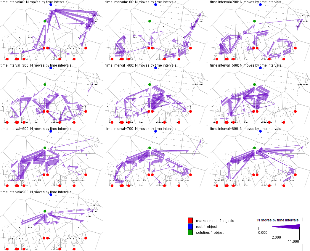
A display consisting of multiple flow maps can be used to represent summarized eye movements in different time intervals or clusters of time intervals, or movements of different users or user groups.
For example, the display below represents a temporal sequence of summarized eye movements. Before aggregating the data, the trajectories have been aligned to the same start and end times; hence, we consider relative time intervals with respect to the whole duration of the task fulfillment (i.e., trajectory duration). We have divided the trajectory duration into 10 equal intervals; hence, each of the small maps represents a time interval of 10% of the task completion time. For clutter reduction, only the flows representing at least two moves are shown.
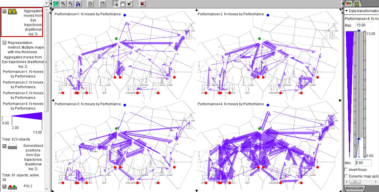
The example display below represents summarized eye movements for four user groups defined according to the performance: (1) 9 fastest users; (2) 9 users from places 10-18 according to the performance; (3) 9 users from places 19-27; (4) 10 slowest users.
On a flow map or a display with multiple flow maps, it is possible to transform the values of the currently represented aggregate attribute to differences from values of another attribute. For each flow, the value of the second attribute is subtracted from the value of the first attribute and the resulting difference is represented by the thickness and color of the flow symbol. Two different (opposite) colors are used to represent positive and negative differences. The widths of the flow symbols are proportional to the absolute values of the differences.
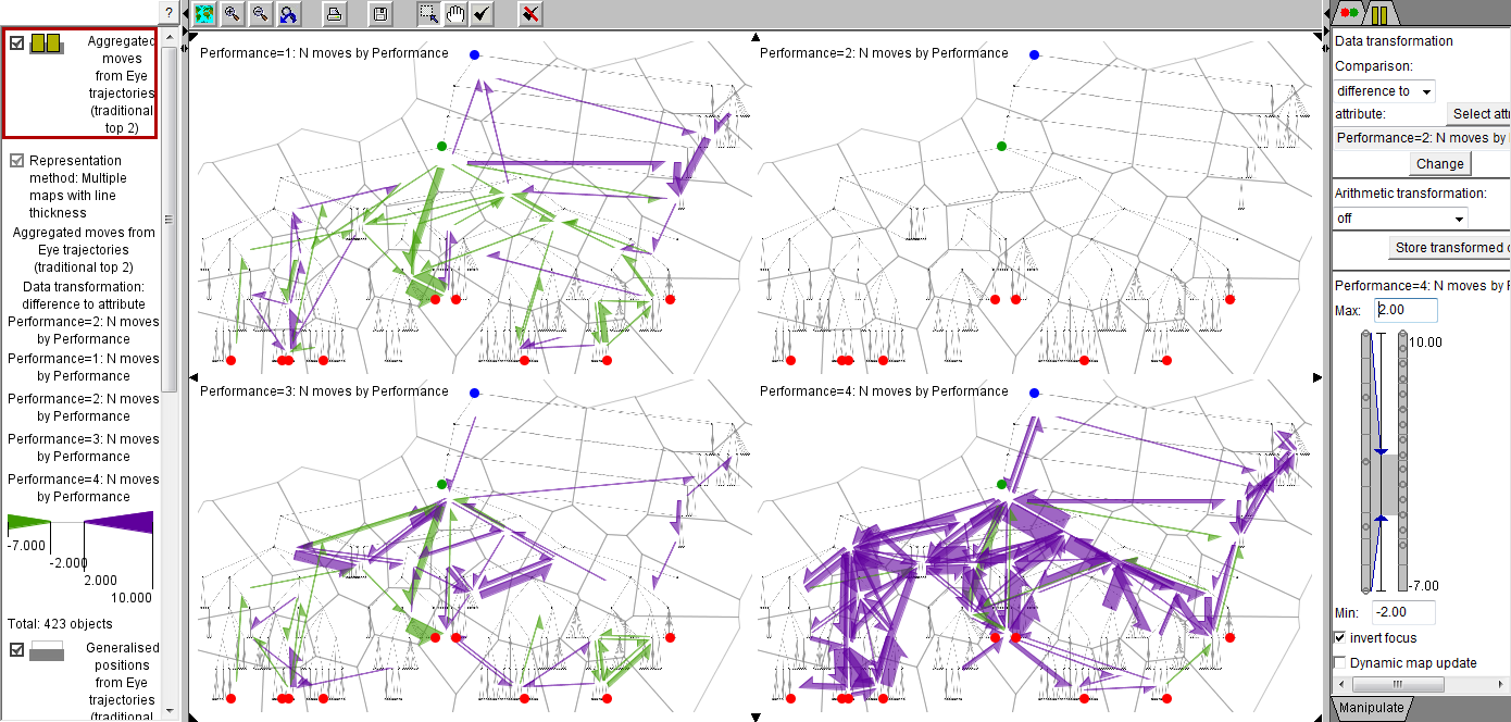
In the example below, we apply this transformation to the multiple flow map display representing summarized eye moves of the four user groups according to the performance. The counts of the second fastest group (group 2) have been subtracted from the counts of all groups. The positive differences in move counts are shown in violet and negative in green. To reduce the display clutter, we have hidden the flows where the absolute differences are less than 2. No flows are visible on the map for group 2 since all the differences are zeros.
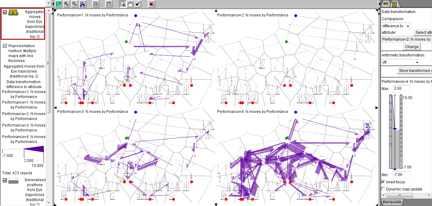
By interactively manipulating the display, it is possible to consider separately the positive and negative differences. In the image below, we see the positive differences from group 2, i.e., where the users from the other groups moved their eyes more than the users from group 2.
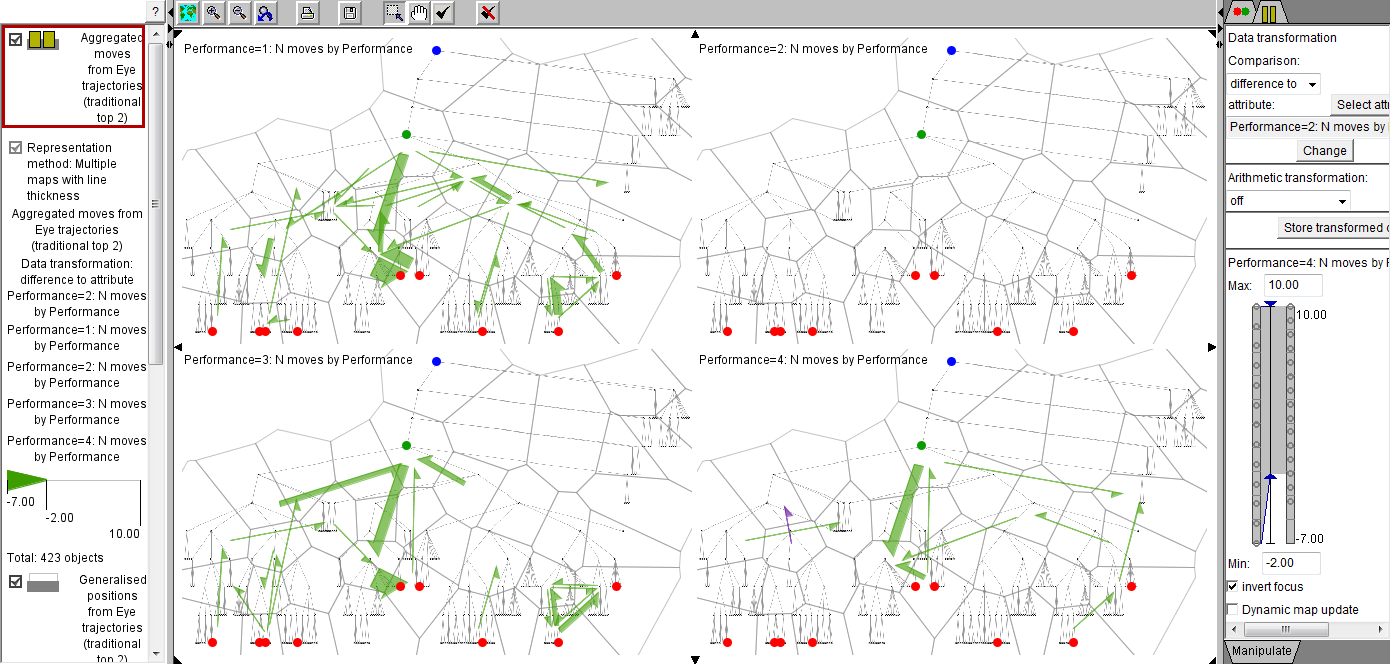
In the image below, we see the negative differences from group 2, i.e., where the users from group 2 moved their eyes more than the users from the other groups.
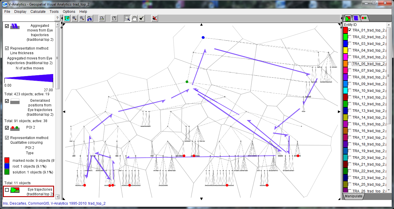
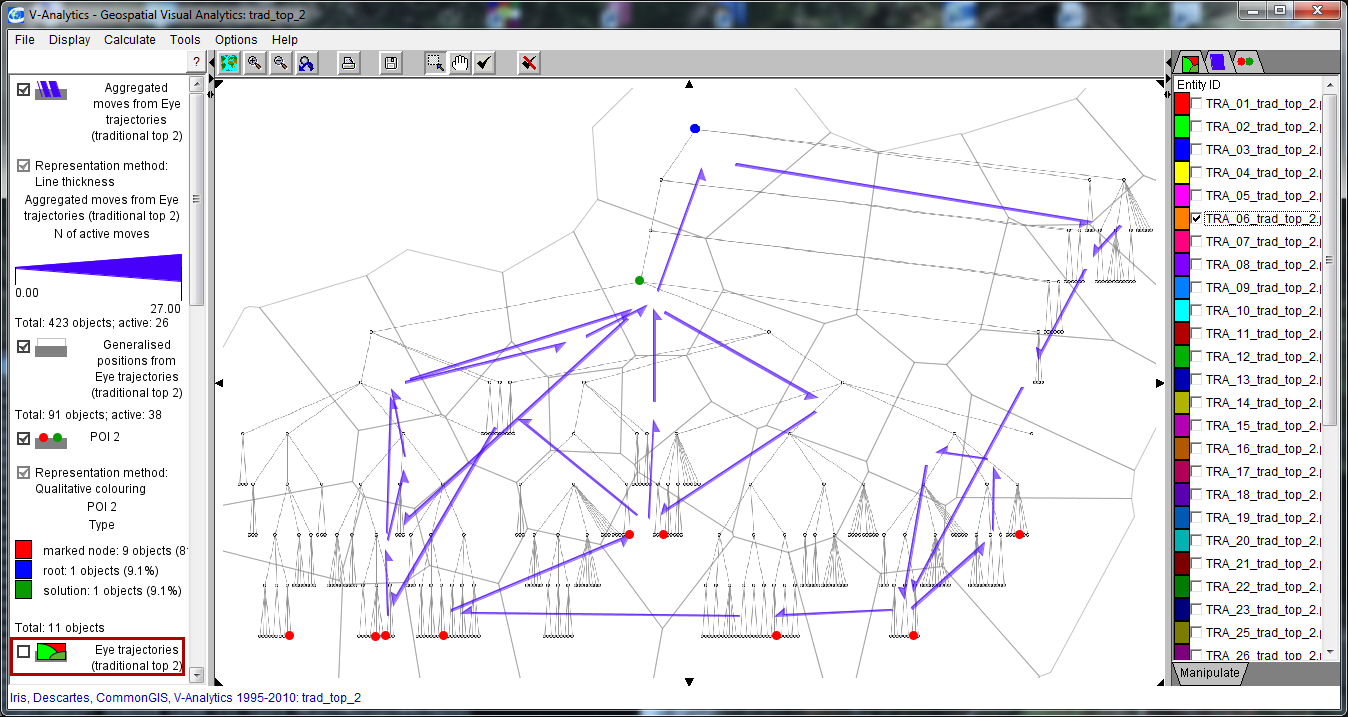
Juxtaposed flow maps show summarized eye movements on different displays.
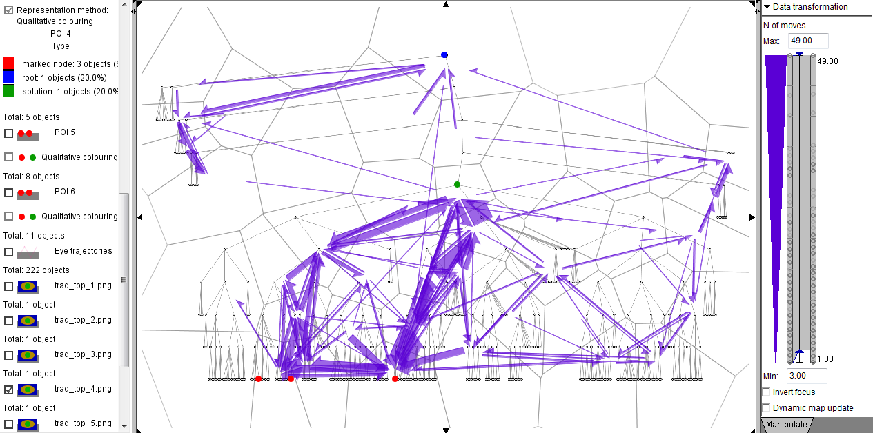
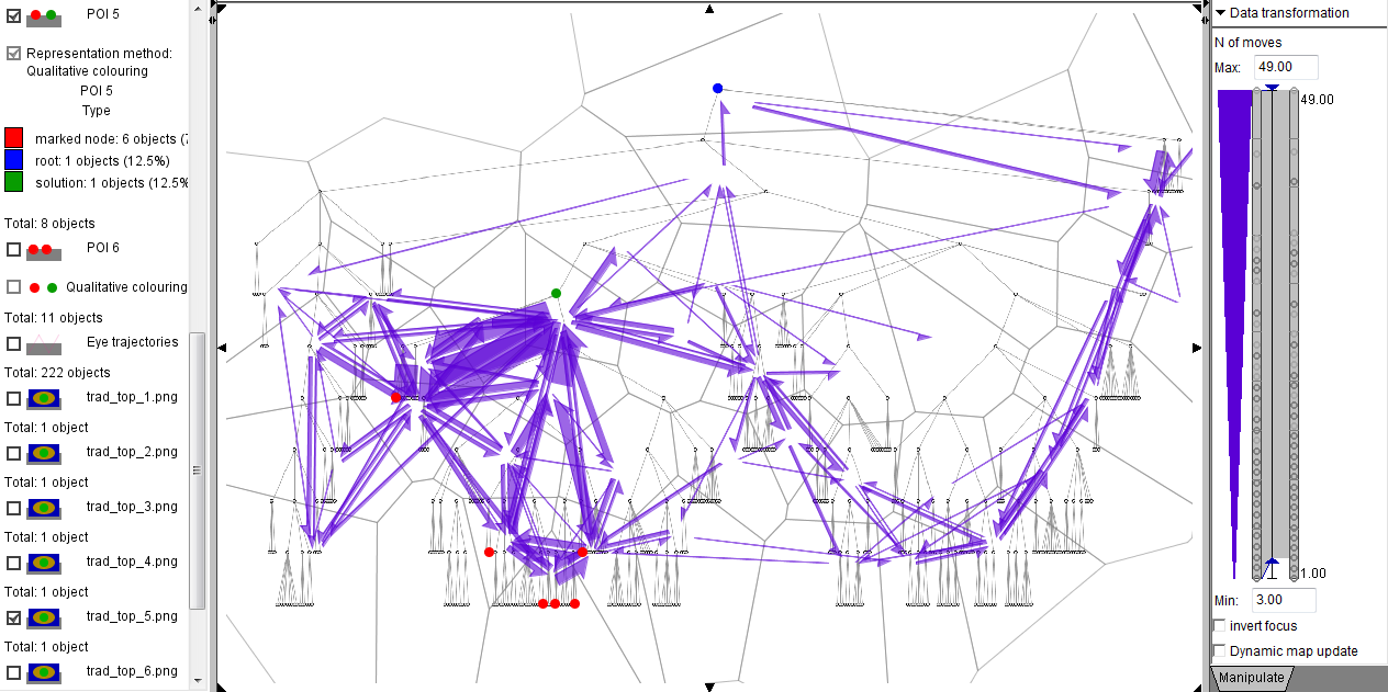
For example, two flow maps below represent the summarized eye movements for two different trees. For clutter reduction, only the flows representing at least three moves are shown.
Natalia Andrienko, Gennady Andrienko
Spatial Generalization and Aggregation of Massive Movement Data
IEEE Transactions on Visualization and Computer Graphics (TVCG), 2011, v.17 (2), pp.205-219
published version:
http://doi.ieeecomputersociety.org/10.1109/TVCG.2010.44
Natalia Andrienko, Gennady Andrienko, Hendrik Stange, Thomas Liebig, Dirk Hecker
Visual Analytics for Understanding Spatial Situations from Episodic Movement Data
Künstliche Intelligenz, 2012
pre-print
published version:
http://dx.doi.org/10.1007/s13218-012-0177-4
Gennady Andrienko, Natalia Andrienko
A General Framework for Using Aggregation in Visual Exploration of Movement Data
The Cartographic Journal, 2010, v.47 (1), pp. 22-40
pre-print