Exploration and comparison of many trajectories can be done using computational estimation of the degrees of dissimilarity (distances) between them. Before comparing trajectories, either visually or by computing distances, it may be meaningful to apply generalization, which removes minor fluctuations.
For measuring the similarity between eye scanpaths, we suggest the “route similarity” distance function, which repeatedly searches for the next pair of closest positions from two trajectories and computes the mean distance between the matching positions plus a penalty distance for the unmatched positions. The penalty distance is the sum of the deviations of the unmatched points from the nearest matched points divided by the length of the matching parts of the trajectories (the mean of the two lengths is taken).
One possible way of path similarity analysis is to compute distances of all trajectories to a selected trajectory (e.g. the fastest one) or a hypothetical optimal trajectory and then analyze how the other trajectories differ from it. Another possible way is to compute pairwise distances, group the trajectories by similarity using a suitable clustering or projection method, and then explore groups of similar trajectories.
One trajectory is selected as a reference. Using the distance function, the distances (i.e., amounts of dissimilarity) of all trajectories to the reference trajectory are computed. Then the closest (most similar) trajectories are viewed one by one.
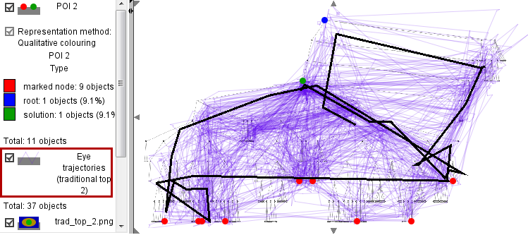
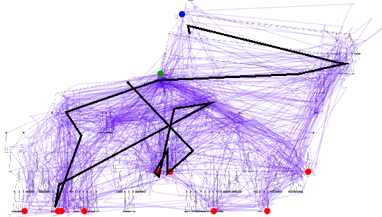
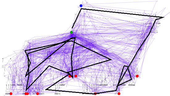
In the example below, we have selected a trajectory whose shape is the closest to the optimal one (an optimal scanpath for the task of finding the least common ancestor of the marked leaf nodes would be to attend only to the leftmost and rightmost marked nodes and disregard the intermediate ones).
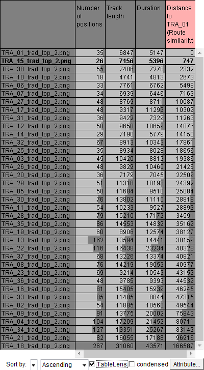
Then the distances of all trajectories to the reference trajecvtory have been computed using the distance function "route similarity". The table on the left shows the computed distances in the rightmost column. The rows, corresponding to the trajectories, are sorted in the order of accending distances to the reference trajectory. We select the trajectories one by one by clicking on the table rows. The selected trajectories are highlighted in black in the map display. The screenshots on the right show four trajectories whose shapes are the most similar to the shape of the reference trajectory.
|
|
Eye trajectories of different users may be very diverse. To estimate how diverse the trajectories are and whether any common viewing or searching strategies may exist, we suggest the following procedure. Using the "route similarity" function, a matrix of pairwise distances between the original or generalized trajectories is computed. This matrix is used to create a two-dimensional projection of the set of trajectories by means of multi-dimensional scaling (MDS) or Sammon’s mapping. Based on the projection obtained, the trajectories can be grouped (clustered) by similarity.
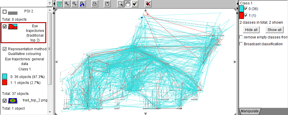
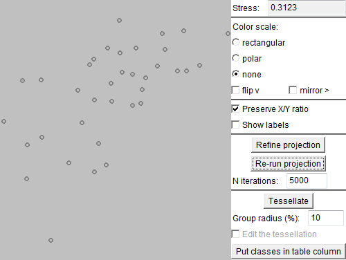
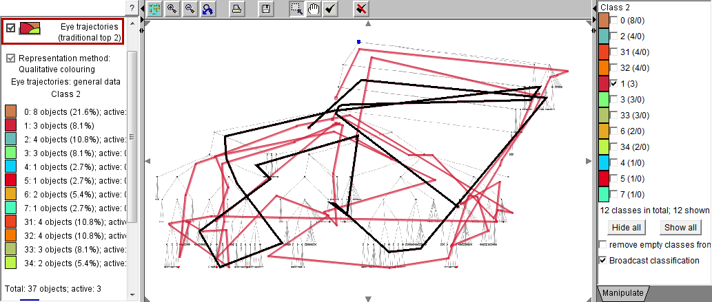
In the images below, we have applied Sammon's mapping to the matrix of distances between 37 eye trajectories. The trajectories are represented by dots (small circles). One trajectory is positioned far from the others, which means that its shape is very dissimilar to the shapes of the other trajectories. The presence of this outlier in the projection complicates the consideration of the remaining points since they are positioned very close to each other. Using the projection, we separate the outlying trajectory from the rest. For this purpose, we divide the projection plot into two regions, which define two classes of trajectories: one consists of the outlying trajectory and the other includes all the rest.
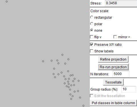

The map on the left shows the two classes of trajectories defined by means of the projection. The map on the right presents the outlying trajectory.

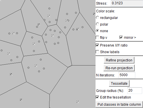
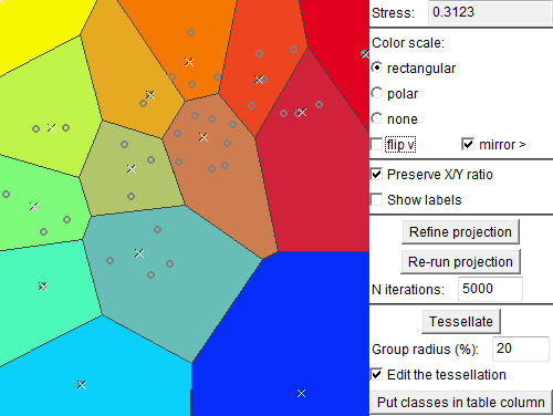
Next, we deselect (filter out) the class consisting of the outlying trajectory and apply Sammon's mapping to the remaining trajectories. By dividing the space of the projection plot into areas, we define groups of trajectories that are close to each other in the projection space, i.e., have similar shapes according to the distance function "route similarity". The areas can be assigned different colors, which are then used for marking the trajectories in various displays. Note that close areas receive similar colors.
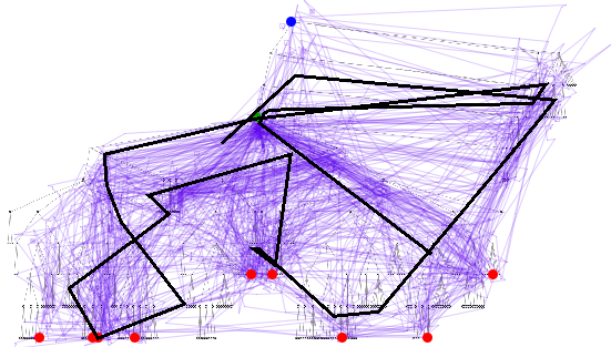
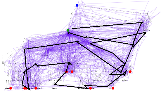
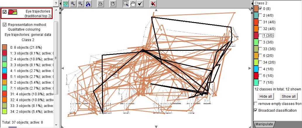
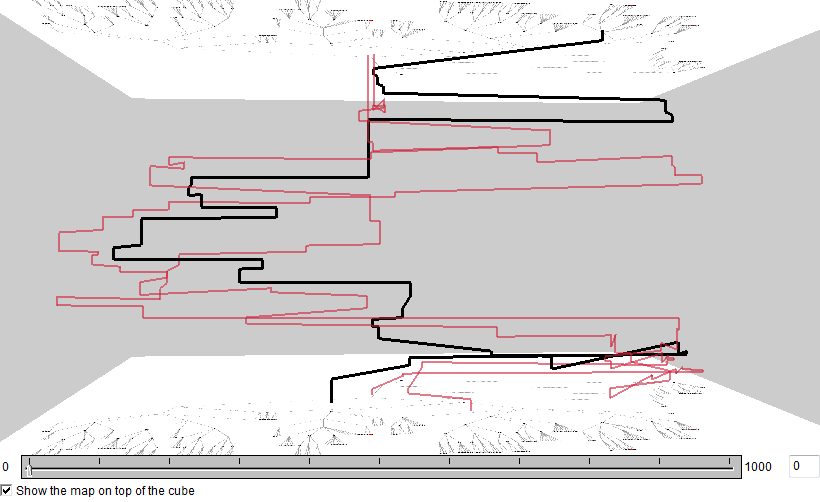
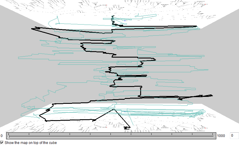
Now the groups (clusters) of trajectories can be selected and explored using a map display of trajectories and/or a space-time cube. The images below represent three clusters. In each cluster, the trajectory that is the closest to the cluster center is highlighted in black. The time references of the trajectories have been adjusted to common start and end times. It can be noted that there is much diversity even within the clusters.


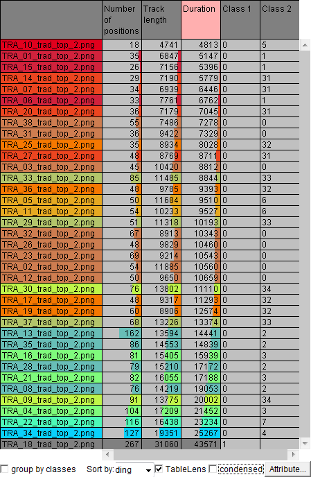
The colors of the clusters can also be used in a table display with attributes of the trajectories. In the table below, the rows are sorted in the order of increasing trajectory duration (i.e., the task completion time). We can see that shades of red prevail at the top of the table and the shades of green and cyan at the bottom. Hence, the upper right corner of the projection plot includes the eye trajectories of faster users and the lower left corner the trajectories of slower users. The last table row, colored in dark gray, corresponds to the outlying trajectory, which has been excluded after the first stage of the analysis.
The distance function "route similarity" is described in the following paper:
Gennady Andrienko, Natalia Andrienko, Stefan Wrobel
Visual Analytics Tools for Analysis of Movement Data