Appendix to Section 6.2
Partition-Based Clustering (K-Means) – EU NUTS-3 Population Structure

The analyst begins Phase 1 of the SI workflow by sweeping the number of clusters from K = 3 to K = 50 with a fixed random seed. The data comprise demographic indicators for ~1,500 European NUTS-3 regions: percentage of female population and distribution across age groups (0–14, 15–24, 25–44, 45–64), with pct_male and pct_65_plus excluded to avoid linear redundancy.

The IteraScope metrics chart reveals a clear silhouette peak at K = 6 with a secondary plateau from K ≈ 18 to K ≈ 24. The SSE curve shows the expected monotone decrease with no sharp elbow. The HDBSCAN archetype detection marks K = 24 as the first complete iteration (all archetypes present); however, K = 20 already achieves a silhouette score close to the plateau maximum and contains all but one archetype.

To compare the two candidate configurations in detail, the analyst examines the Sankey transitions between K = 20 and K = 24. The first view below shows the full transition pattern: most groups at K = 20 persist as single groups at K = 24, with a few splitting into two or more sub-clusters. The violet cluster (20.10) is of particular interest—it maintains strong band continuity toward cluster 24.7.

The analyst then focuses on cluster 20.10 specifically, using the "highlight transitions from" interaction to visualise all outgoing flows from this group to K = 24. The Sankey view confirms that the vast majority of members persist in cluster 24.7, with only thin bands splitting off to adjacent clusters (24.3, 24.11, etc.).

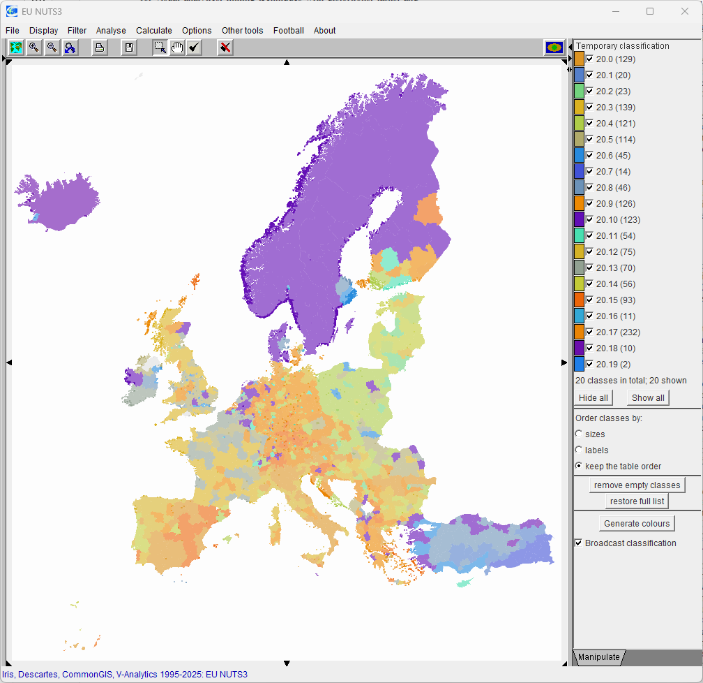
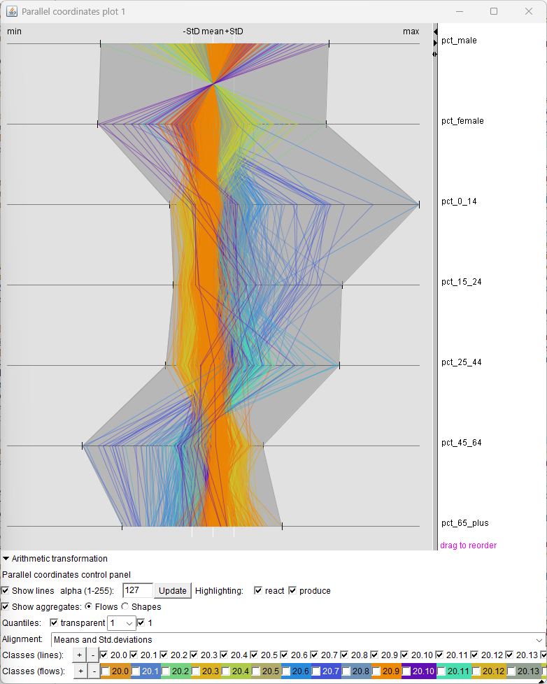
The analyst shares the K = 20 grouping to the linked map and parallel coordinates to assess geographic coherence and demographic interpretability. The map reveals clearly delineated regional typologies: Nordic, Mediterranean, Central-European, and Eastern-European patterns are visible as spatially contiguous clusters. The parallel coordinates plot shows well-separated multivariate profiles for each cluster.

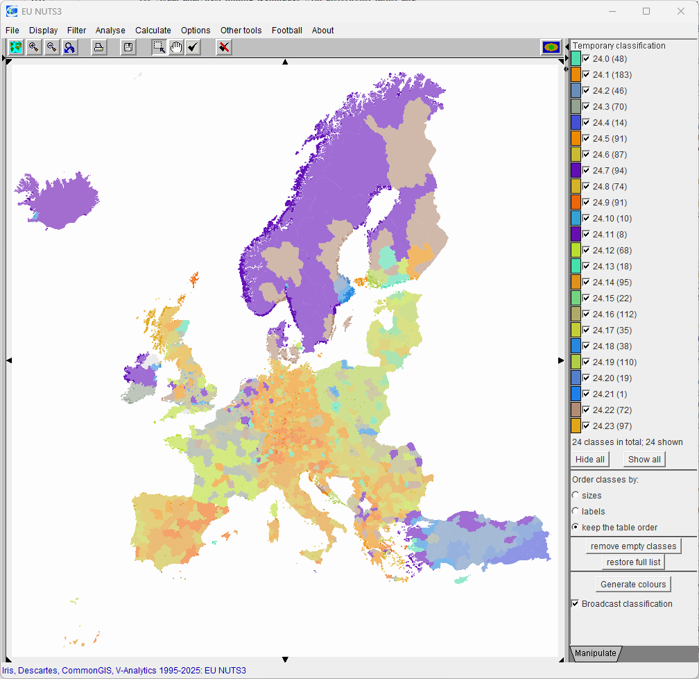
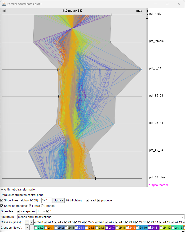
For comparison, the analyst also shares the K = 24 grouping to the same linked views. The map shows similar macro-level patterns but appears visibly more scattered: several spatially coherent regions from K = 20 are now fragmented without clear interpretive gain. The parallel coordinates plot confirms that the four additional clusters do not introduce qualitatively new demographic profiles—they subdivide existing ones along cluster boundaries.

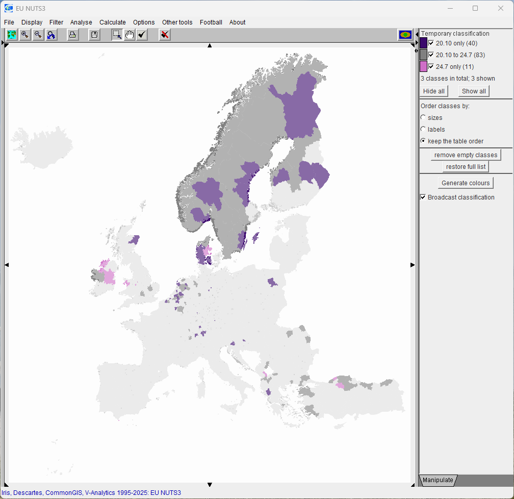
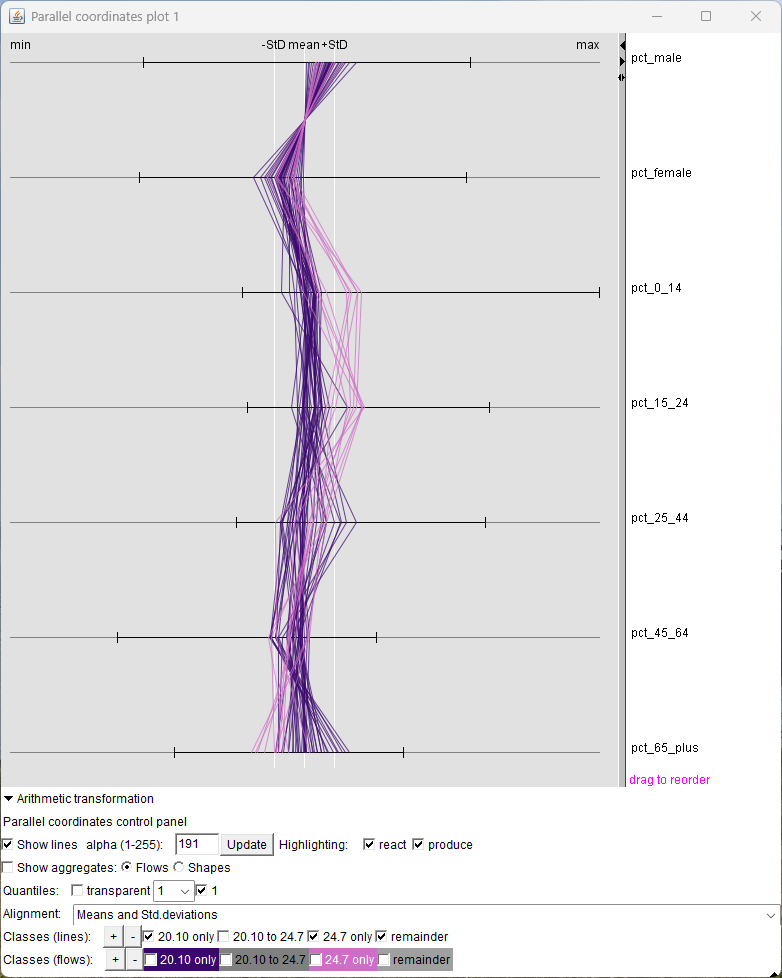
The analyst highlights the specific transition from cluster 20.10 to cluster 24.7 and propagates the resulting class attribute to the map and parallel coordinates. This isolates the members that persist in the violet cluster when K increases from 20 to 24. The map confirms that the retained members form the spatial core of the cluster—a contiguous mass across Scandinavia and the Baltic coast. The parallel coordinates plot shows that the demographic profile of this core is even more sharply defined than the full cluster at K = 20, since borderline members with intermediate profiles have been excluded.

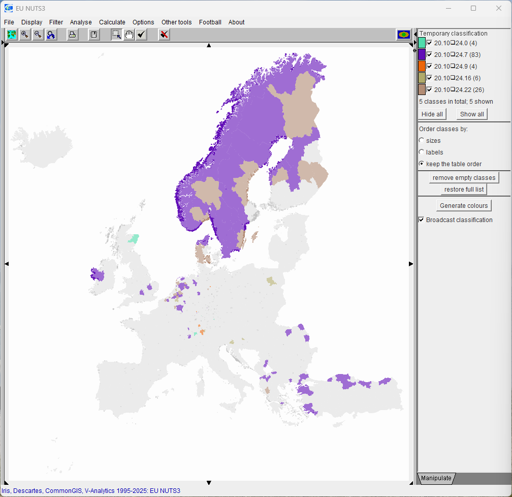
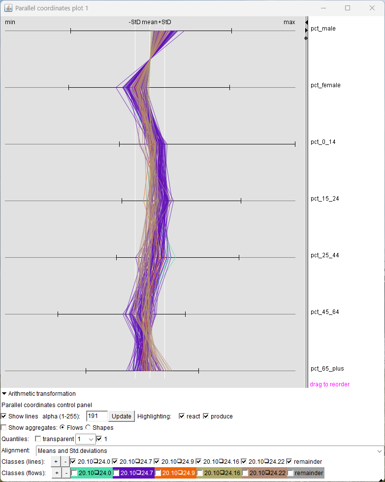
Next, the analyst highlights the transition from cluster 20.10 to all clusters at K = 24, creating a class attribute whose values encode each destination ("20.10 → 24.7", "20.10 → 24.3", "20.10 → 24.11", etc.). This decomposition reveals where the "lost" members go. The map shows that members reassigned away from the violet cluster are scattered along its geographic boundary—they are absorbed into geographically adjacent clusters rather than forming a single coherent new group. The parallel coordinates confirm that these boundary members have intermediate demographic profiles: they share characteristics of both the violet cluster and their new host clusters.

To verify that the K = 20 solution is not an artefact of a particular random initialisation, the analyst reruns K-Means with K = 20 fixed and sweeps the random seed from 1 to 30. This round addresses Phase 5 of the SI workflow: archetype verification and robustness assessment.

The IteraScope display shows remarkable consistency across seeds. The Sankey bands between consecutive seeds are almost perfectly horizontal—indicating no splits or merges. Silhouette fluctuates by less than 0.01 across all 30 seeds. The 2D embedding shows tight archetype clusters with negligible seed-to-seed drift, confirming that the cluster structure at K = 20 is determined by the data geometry rather than by the random initialisation.

Seed 1 is selected as the reference solution because: (i) none of its 20 clusters falls into HDBSCAN noise—indicating that every cluster possesses sufficient density and coherence; and (ii) the iteration is marked as complete, confirming that all recurrent archetypes are represented.

The table below summarises the two rounds of the partition-based clustering workflow, showing how each round addressed specific analytical questions within the SI workflow framework.

Final selected parameters: K = 20, seed = 1. This configuration produces 20 clusters capturing distinct European demographic typologies—including an ageing northern-European profile (violet cluster), young Mediterranean and Eastern-European profiles, and urban/metropolitan profiles—with high membership confidence, strong geographic coherence, near-complete archetype coverage, and full robustness to random initialisation.